Reinforcement Learning

Agents receive feedback from the environment in the form of rewards
Utility of the agent is defined by the reward function
Goal is to maximize expected future reward using only observations/interaction with the environment
We still assume an MDP, but now we don’t know the true transition $T$ or reward function $R$ , and we have to actually try actions and make observations to learn them

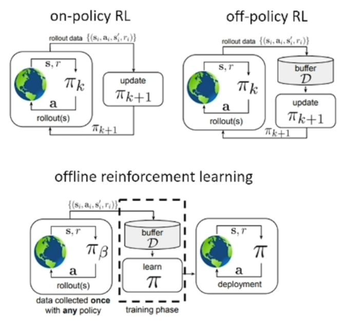
On-policy RL

On-policy learning is considered the more conventional approach to RL. In this setting we simply have our policy suggest actions that are taken by the agent, and the observed data is then used to update the policy. Here we are always staying “on policy” as we’re only ever learning along a trajectory suggested by the policy itself.

Off-policy RL

Off-policy learning describes the setting where a policy is able to learn from data collected by a number of policies. These methods still collect additional data as they go; for example, a policy could collect a number of observations, store them in a buffer, and learn from the entire buffer before advancing another step.

Offline RL

Offline learning takes place in the setting where our policy has no active interaction with the environment during the training phase. Instead, we have a dataset available a priori, collected by a typically unknown policy (e.g. could another RL policy, could be humans, etc), and our goal is to learn a policy strictly from this already available dataset alone.

Model-based Learning

Model-based learning approaches RL by learning an approximate model of the environment using observations
More specifically, we build an empirical MDP model, and then solve the learned MDP:
- Step 1: Learn empirical MDP
  - Count outcomes $s^\prime$ for each $s$ , $a$
  - Normalize to get estimate $\hat{T}(s,a,s^\prime)$
  - Keep track of experience rewards $R(s,a,s^\prime)$
- Step 2: Solve learned MDP
  - Here we can use techiniques seen previously like value iteration

Model-free Learning

Passive Reinforcement Learning

Given a fixed policy $\pi(s)$ , we want to learn state values by following this policy passively. The agent has no choice regarding the actions that it takes, but it can still learn from the states in encounters.
This is different from online planning, as we are actually taking actions in the real world

Direct Evaluation

Goal is to compute state values under a given policy $\pi$ . When acting according to $\pi$ , each time a state is visited we compute and keep track of what the sum of discounted rewards turned out to be.
Called direct evaluation for obvious reason, we are directly evaluating what the rewards are as we experience them

Tradeoffs

Beneficial in that it’s easy to understand, doesn’t require prior knowledge of $T$ or $R$ , and eventually recovers the correct values
Bad because it wastes information about state connections, and takes a long time to converge properly since each state must be learned separately

Sample-Based Policy Evaluation

Policy evaluation enabled us to evaluate state values under a given fixed policy: $V_{k+1}^{\pi_i}(s) \leftarrow \sum_{s^\prime}T(s,\pi_i(s),s^\prime)\big[R(s,\pi_i(s),s^\prime) + \gamma V^{\pi_i}_k(s^\prime)\big]$
To estimate this we can take samples of outcomes and average: $\text{sample}_i = R(s,\pi(s),s_i^\prime) + \gamma V_k^{\pi}(s^\prime)$ $V_{k+1}^\pi(s) \leftarrow \frac{1}{n}\sum_i{\text{sample}_i}$

Temporal Difference Learning

Here we update $V(s)$ $V (s)$ every time a transition $(s,a,s^\prime,r)$ $(s, a, s^{'}, r)$ is observed. Here the policy is still fixed.
- Sample of $V^\pi(s)$ : $\text{sample} = R(s,\pi(s),s^\prime) + \gamma V^\pi(s^\prime)$
- Update to $V^\pi(s)$ : $V^\pi(s) \leftarrow (1-\alpha) V^\pi(s) + \alpha\cdot\text{sample}$
This update process corresponds to an exponential moving average, which forgets about the past in preference for new information (old values were wrong anyway)
TD learning is model-free way to do policy evaluation, but can’t easily turn value estimates into a policy. So learn q-values instead

Q-value Iteration

Basic principle is that q-values are more useful, so use value iteration but compute q-values instead
Start with $Q_0(s,a)=0$ , and compute depth $k+1$ q-values given $Q_k$ $Q_{k+1}(s,a) \leftarrow \sum_{s^\prime}T(s,a,s^\prime)\big[R(s,a,s^\prime) + \gamma \max_{a^\prime}Q_k(s^\prime,a^\prime)\big]$
Of course, we don’t have the real $T$ $T$ or $R$ $R$ functions, so we compute $Q(s,a)$ $Q (s, a)$ as we go. Known as Q-learning:
- Receive sample $(s,a,s^\prime,r)$
- Compute new sample estimate $\text{sample} = R(s,a,s^\prime) + \gamma \max_{a^\prime}Q(s^\prime,a^\prime)$
- Incorporate new estimate into running average: $Q(s,a) \leftarrow (1-\alpha)Q(s,a) + \alpha[\text{sample}]$
Q-learning converges to optimal policy even when acting suboptimally, known as off-policy learning

Q-learning: Recap

Want to perform Q-value updates to each Q-state

$Q_{k+1}(s,a) \leftarrow \sum_{s^\prime}T(s,a,s^\prime)\big[R(s,a,s^\prime) + \gamma\max_{a^\prime}Q_k(s^\prime,a^\prime)\big]$

However this can’t be computed without knowing $T$ and $R$ , which we do not have in the typical online reinforcement learning scenario. So what do we know?

When a sample transition $(s,a,r,s^\prime)$ is observed, we have evidence which suggests that $T(s,a,s^\prime) \approx 1$ and $R(s,a,s^\prime) \approx r$ . Thus, we have the approximation

$Q(s,a) \approx r + \gamma\max_{a^\prime}Q(s^\prime,a^\prime)$

As we observe more sample transitions, however, this approximation can be updated via a running average:

$Q(s,a) \leftarrow (1-\alpha)Q(s,a) + (\alpha)\big[r+\gamma\max_{a^\prime}Q(s^\prime,a^\prime)\big]$

where $\alpha$ is a some weighting parameter. The higher $\alpha$ is, the more we accentuate recent sample transitions and thus learn faster, but at the detriment of stability.

Properties

Q-learning converges to the optimal policy, even when we start out acting suboptimally. This is what’s known as off-policy leaning. Note that this property assumes that you “explore enough,” and eventually make the learning rate sufficiently small.

Exploration vs Exploitation

Fundamental tradeoff of reinforcement learning: to follow the currently best known policy (exploitation), or try a new policy in hopes of coming across something even better (exploration)?

Can explore using $\epsilon$ -greedy random actions: select with some small probability $\epsilon$ a random action, $1-\epsilon$ act according to current policy
Lowering $\epsilon$ over time can reduce random bad actions after state space is sufficiently explored

Exploration Functions

Help decide where to explore and for how long
Exploration functions take value estimate $u$ and visit count $n$ and return an optimistic utility $f(u,n) = u+k/n$

Regret

Regret is the measure of total mistake cost, the difference between expected rewards and the optimal expected rewards
Minimizing regret is done by optimally learning to be optimal, minimizing the amount of mistakes along the fail
For example, random exploration has higher regret than using exploration functions despite both ending up optimal

Generalizing Across States

Realistically can’t keep table of all q-values, too many states
Want instead to generalize from a few training states (fundamental ML concept)
Can use feature-based representations, i.e. describe a state with a vector of features

Approximate Q-learning

With a feature representation, can write a q, or value, function for any state with a few weights. Call these linear value functions: $V(s) = w_1f_1(s) + \cdots + w_nf_n(s)$ $Q(s,a) = w_1f_1(s,a) + \cdots + w_nf_n(s,a)$
Q-learning with linear Q-functions
- Observe transition $(s,a,r,s^\prime)$
- Difference equal to $\big[r+\gamma_{a^\prime}Q(s^\prime,a^\prime)\big] - Q(s,a)$
- Exact Q’s: $Q(s,a) \leftarrow Q(s,a) + \alpha[\text{difference}]$
- Approx Q’s: $w_i \leftarrow w_i + \alpha[\text{difference}]f_i(s,a)$
- This approximate update comes from online least squares, where we find the gradient of the squared error w.r.t. our weight

Policy Search

Often feature-based policies that work well don’t necessarily correspond to good esimates of values and q-values
We want to learn policies that maximize rewards, not the values that predict them
Simple policy search starts with initial linear value or Q-value function, make small changes to weights up and down and see if policy is better than before

Learning methods

Policy gradient

Goal is to learn a policy $\pi_\theta(a_t|s_t)$ , a conditional distribution over the actions at time $t$ given state $s_t$ . $\theta$ represents the parameters of the model that represents the policy, and is typically taken as the weights of a neural network. So this neural network takes $s_t$ and outputs the conditional probability distribution $\pi(a_t|s_t)$ .

The overall learning objective is here is to find the policy which maximizes the expected sum of discounted rewards over a given action horizon. That is,

$\text{max}_\pi \sum_{t=0}^T \mathbb{E}_{s_t \sim d^\pi(s),a_t\sim\pi(a|s)}[\gamma^t r(s_t,a_t)]$

We define $J(\theta)$ to be this inner sum of discounted rewards under a policy $\pi_\theta$

$J(\theta) = \mathbb{E}_{\tau\sim\pi_\theta(\tau)}\Big[\sum_{t=0}^T \gamma^tr(s_t,a_t)\Big] \approx \frac{1}{N}\sum_{i=0}^N\sum_{t=0}^T \gamma^tr(s_{t,i},a_{t,i})$

where on the right we’ve shown an approximate computation of $J$ one might make in practice after observing $N$ rollouts. The policy gradient method is then interested in computing the gradient of $J$ with respect to parameters $\theta$ , essentially giving us a way of changing the network parameters to yield the fastest increase in the value of $J$ . We can use this idea to iteratively improve our policy and maximize our expected sum of discounted rewards. This gives rise to the classic REINFORCE algorithm:

Sample trajectory $\tau_i \sim \pi_\theta(a_t|s_t)$ by running the policy
Compute the gradient $\nabla_\theta J(\theta) \approx \sum_i\Big(\sum_t\nabla_\theta\log\pi_\theta\big(a^i_t|s^i_t\big)\Big)\Big(\sum_tr\big(s^i_t,a^i_t\big)\Big)$
Perform simple gradient descent update $\theta \leftarrow \theta + \alpha\nabla_\theta J(\theta)$

Reinforcement learning