sbi package
SBI Python packageThe sbi Python package is a toolbox for Simulation-based inference. It makes use of three main Machine learning methods to approach the problem:
- Sequential neural posterior estimation (SNPE)
- Fast free inference of simulation models: seems to introduce the core neural pipeline for modeling the posterior using a neural network (particular a mixture-density network). It pairs this with a continuously updating proposal prior (being set to the current estimate of the posterior after each batch of simulated samples), and ultimately hopes to converge on a mixture distribution sufficiently similar to the posterior distribution.
- Flexible statistical inference for mechanistic models: feels very much like an like the paper in (a), introducing (?) the exact the same pipeline for modeling the posterior. It applies this specifically to neural dynamics models, which are literally models of neural circuitry in the brain. It looks like they tack on some extra methods for handling missing features when the simulator fails and learning relevant features with RNNs.
- Automatic Posterior Transformation for Likelihood-free Inference: introduces Automatic Posterior Transformation (APT), new sequential neural posterior estimation for SBI. Papers mentions hopes to overcome problems in (a), including restricted proposals and instability of needing importance weighting. APT can modify posterior estimate with “arbitrary, dynamically updated proposals,” and can operate “directly on high-dimensional time series and image data.”
- Sequential neural likelihood estimation (SNLE)
- Sequential Neural Likelihood: introduces new method for learning likelihood directly. Main idea of SNL is training a “Masked Autoregressive Flow” (think PixelCNN) to simulate the conditional density of data given parameters (i.e. the likelihood). This is paired with an MCMC sampler which selects the next simulations to run using dynamically updated estimates of the likelihood function (not unlike the above methods, where the posterior estimate in a previous step becomes the proposal for the next step).
- Sequential neural ratio estimation
- Likelihood-free MCMC with Amortized Approximate Likelihood Ratios: approaches SBI by approximating the likelihood-to-evidence ratio. The ratio estimator is then used in methods like the Metropolis-Hastings algorithm to “approximate the likelihood-ration between consecutive states in the Markov chain”. The algorithm has a acceptance ratio dependent on the likelihood, and the paper attempts to remove this dependency by modeling the ratio directly with an amortized ration estimator.
According to the documentation, one of these approaches should be most suitable to the problem at hand depending on certain properties (namely the sizes of the observation space and the parameter space).
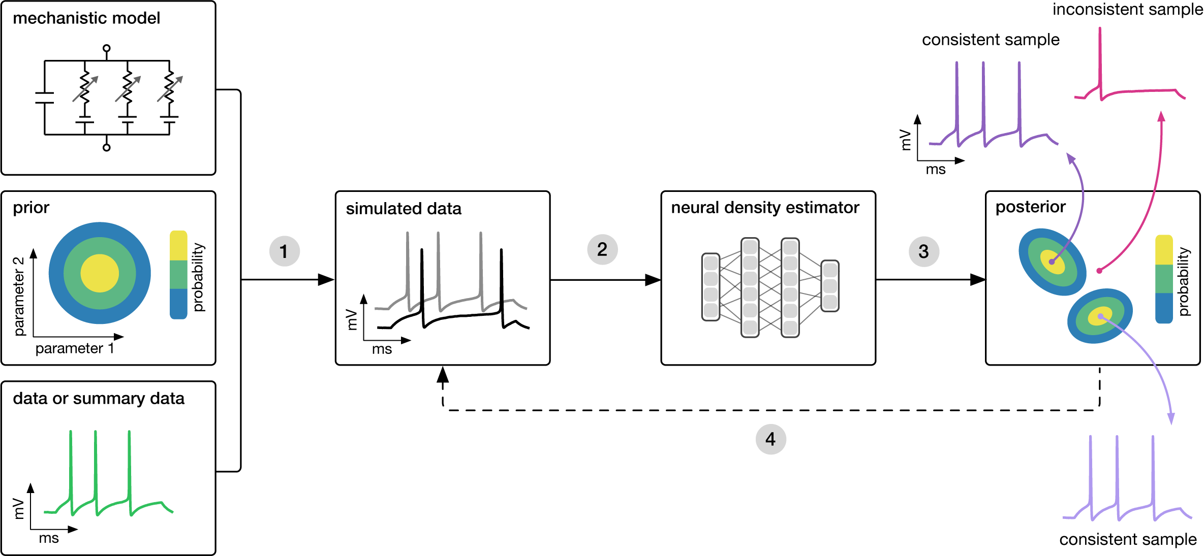
The following figure outlines visually the process of algorithmically identifying models that are consistent with some real world observations.
Package usage
To begin, you must have the basics of your environment set up and defined. This includes at the minimum (1) a prior over the parameter space from which to pull simulator parameter values, and (2) the simulator itself, producing simulated data after taking a set of parameters. Since Simulation-based inference is a method for finding parameter values of a simulator that produce outputs matching real world observations, you will later need the actual observations you wish to condition the posterior on.
A simple example from the docs is broken down as follows:
num_dim = 3
prior = utils.BoxUniform(low=-2*torch.ones(num_dim), high=2*torch.ones(num_dim))
Here we define our prior distribution, a 3D uniform box-like density ranging from [-2, 2] on each axis. This is the space from which we will sample our 3-dimension parameter vector , parametrizing the simulator defined below:
def simulator(parameter_set):
    return 1.0 + parameter_set + torch.randn(parameter_set.shape) * 0.1
This simulator takes the parameter vector, shifts it by 1, and adds a small amount of Gaussian noise before returning this value as an output. This example makes it very clear to see how the parameter values impact the value of the output (albeit with some added stochasticity), but with virtually any other simulator this relationship will be much more complex and indirect. This simulator also defines the explicit likelihood
This is usually the intractable piece that makes simulation based inference difficult, but for the sake of example we have a known, closed form. We then run inference using our defined components:
posterior = infer(simulator, prior, method='SNPE', num_simulations=1000)which will, in the case of SNPE, train a neural network (neural density estimator) on samples, where (the prior defined earlier), and (the likelihood defined by the simulator).